1. Geometry Considered.
Geometry studies the spatial arrangements of shapes (lines, polygons, circles, ... ).
"Statistical" and "geometry" are words not usually seen together, so some explanation of this much-neglected subject is called for.
Geometry is a huge and ancient subject. In art and decoration certain branches of geometry have been much used. Tilings of the plane go back a long way, are pleasing to the eye, and have been especially prominent in Islamic art and decoration. Plane tilings are also widely seen in quiltmakers work. Such tilings pose the question "How do you fill the plane without gaps using a limited number of geometric shapes?" -- typically polygons or other simple shapes bounded by straight lines. The result is a pattern which covers some bounded region with a finite number of shapes.
A related area of geometry is that of "packings" -- incomplete or maximally-dense filling of a region by circles and other simple shapes. Circle packings alone have a large mathematical literature. The usual rule in circle packings is that one finds a set of circles which all touch (are tangent to) each other. Such tangent packings are called "Appolonian" after an ancient Greek mathematician (Appolonius of Perga) who first described such a pattern. Such packings don't fill the whole region. These packings have seen relatively little use in art. The packings of interest here are non-Appolonian and violate all the rules of formal mathematical circle packing.
Traditional decorative geometric patterns are models of order and regularity, with every shape having an exact location and no elements of randomness.
One might ask: "Can you cover a bounded region with an infinite number of regular shapes?" Several examples of this are known, such as the Sierpinski carpet, but they have found little use in art, perhaps because their appearance is not particularly attractive to the average eye. Such constructions are largely recursive.
The geometric construction described here poses a different question: "How do you cover a bounded region non-recursively with an infinite number of ever-smaller randomly-placed simple shapes (triangles, squares, circles) such that in the limit they completely fill it?" Despite much searching, I have not found any account of a similar algorithm. It appears to be a first.
Geometry is a subject of great exactitude. There are precise rules for edges, angles, and vertices. There is no place for randomness or uncertainty. But if you look at the pictures hanging on the wall of an art museum what you see combines elements of both randomness and order. A street scene, for example, has the regular structures of streets and buildings, and the turbulent swirl of vehicles and pedestrians. There is an attractiveness to an image which combines elements of both order and randomness. Nature itself combines randomness and order. All oak trees have a regular branching structure which the eye easily recognizes. But the details differ from one tree to another in a random way.
The geometry described here would shock and horrify Euclid.
Conventional tilings have exact symmetry -- it is one of their charms. The shapes making up the pattern have rotation, translation, mirror, and other symmetries. The statistical geometry patterns of interest here have individual shapes with symmetry (square, circle, etc.) but there is no symmetry at all in their placement. What they do have is what might be called fractal symmetry (or "statistical self-similarity") -- a regular progression in the sizes of the shapes. The eye recognizes this kind of symmetry. Apparently even untrained observers see this, although they don't know what to call it.
Coloring is an interesting and important matter for tilings and other geometric art. The effect on the viewer can be quite different for different color schemes. The number of possible regular ways of coloring a given pattern is another area with a substantial mathematical literature ("color symmetry").
2. Examples.
This is sliced from a larger image. The smallest squares are barely resolved.
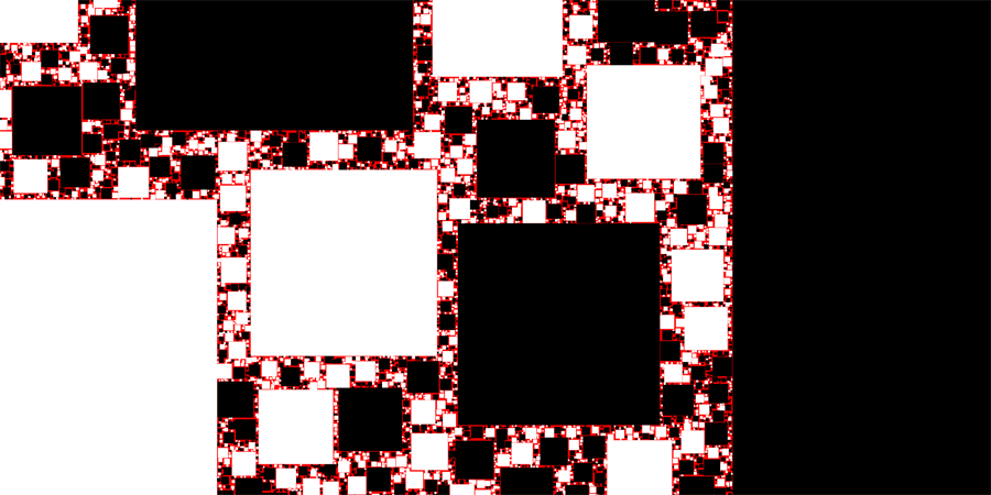
I have done much experimentation with color schemes. The two regions one has are "the squares" and "everything else" (the background or "gasket"). If you use two colors for these regions the image is not very interesting. The squares tend to completely dominate and merge together visually into a blur. The eye has trouble picking up the narrow, fragmented "gasket".
Here the original plane was red, and the squares have been drawn onto it in alternating black and white. Red has enough contrast with both black and white that one can better grasp the overall picture. A pattern of squares of the same color is simply a uniform region. Only when we mark the squares with different colors as in a checkerboard do we see the pattern. This image is in some ways the fractal equivalent of a checkerboard. There is no fundamental difference between the black and white squares.
It may seem to the viewer that the black and white squares are "clustered" into regions more-black and more-white. This is simply randomness in action. If you have this many squares the probability of their clustering is not small. In coin tosses the probability of getting 2 heads or 3 heads in a row is high enough that you see it fairly often if you do a lot of tosses. The apparent clustering here is essentially the same kind of random behavior.
The red region is only about 3 percent of the whole area here. The power-law exponent for the area is 1.40.
If you stare long enough you will see the "statistical self-similarity" in this image. If you look at smaller regions they look just like scaled-down versions of larger regions. This is a key property of fractal patterns.

Here we see a pattern of fractal circles. The original high-resolution file contained 250000 of them but the smallest ones are not resolved here.
Given that the object is to get the viewer to see all of the circles, the right color scheme is quite important. This is another approach. On a whim I tried a version with the colors completely random. It (surprisingly) was a significant improvement on other schemes. This is the version shown here.
The vacant or "gasket" region is a neutral gray.
Application A possible use for this.
3. Rules of Construction.
Suppose that we have a bounded region of area A. We then intend to fill it with similar geometric shapes having a sequence of areas A1, A2, ... (to infinity). The areas Ai are to be computed using a mathematical rule with no randomness.
The algorithm begins by placing shape A1 somewhere within the region. It then proceeds to generate random positions x,y within the region for the following shapes in the sequence, and for each one tests whether any previous Aj overlaps with the given shape Ai. If it does not overlap, this is a "successful placement" and x,y and the area Ai are placed in a file and the process repeated for the next shape A(i+1).
If the shapes are to completely fill the area A in the limit, it is evident that one must have
A = A1 + A2 + A3 + ... (to infinity) Eq. (1)
The area of the ith shape Ai is to be chosen according to some mathematical rule. It is evident that the rule must be such that the sum above is convergent. The sequence of areas Ai should follow some ever-smaller rule: Ai = g(i) for the ith shape.
Several functions obey the obvious requirements: exp(-a*i), exp(-a*i^2), and power laws i^-c where c must be > 1 (the sum in Eq. (1) diverges for c<=1.) Here a and c are parameters which need to be chosen such that Eq. (1) is satisfied.
If the sum in Eq. (1) is less than A, the region will never be completely filled. If the sum is > A, the process of seeking random unoccupied positions for ever-smaller shapes will come to a halt at some point for lack of space.
Power-law functions such as Ai = A1*i^-c (exponent c) are the only ones which have been found to work in computer trials. The "tailing off" of g(i) must be slow enough that there is always room in the lacy "gasket" of unoccupied space for another placement. The gasket must get narrower at just such a rate that allows this.
For a power law Eq. (1) becomes
A = A1 [1 + 1/2^c + 1/3^c + ... (to infinity)] Eq. (2)
The sum in square brackets [ ] can be recognized as the series which defines the Riemann zeta function so that
A = A1 zeta(c) Eq. (3)
For this case with a given choice of A1, it is straightforward to find c
c = zeta_inv(A/A1) Eq. (4)
where zeta_inv is the inverse zeta function. Thus this process does not have a unique power law exponent, but rather an exponent which varies depending on the choice made for the ratio of A1 to total area A. It may be that this is the first-ever practical application of the Riemann zeta function.
In the above calculation it is assumed that all shapes will be placed completely inside the bounded area A. This is easy to do computationally. Other choices such as periodic or cyclical arrangements are possible but so far unexplored.
It has been found that the process also works if the sequence in Eq. (2) does not begin with i=1, but starts with some higher value of i. Or one can have various laws for Ai versus i for the first N terms and then go over to a power law for i>N, as long as Eq. (2) is satisfied.
The process has been used with circles, squares, nonsquare rectangles, and equilateral triangles. The process has been found to run smoothly when set up as described.
By construction the shapes are non-touching (non-Appolonian). With finite-accuracy computing they sometimes touch and may even seem to be slightly overlapping in images. This results from fiinite precision and roundoff error.
4. Observed Properties.
The remarks here apply to the case where one starts with i=1 as in Eq. (2).
This process operates within a very narrow window. For a given choice of A and A1 there is only one value of c which works.
It isn't obvious to me why a power law is the unique choice here. Perhaps a rigorous proof of this is possible for this simple "model" system.
While the total area of the shapes has been set up to go to a particular limit, the perimeter grows without limit as i increases. This is characteristic of fractal patterns.
It has been found in computational experiments that the process does seem to run on "forever" if a power law is used as described above. Sequences of up to 500000 shapes have been computed in this way with no sign that the process will quit (but it does slow down a lot). If the process described here is viewed as a way of measuring area, it reveals a rather surprising property of space.
The process uses random iterations of x,y to find a successful placement. The total (cumulative) number of iterations <nit> needed follows an increasing power law in i, <nit(i)> = n0*i^f, with an exponent f. Study of computed data shows that f = c, i.e., the (negative) value of c is the same (within statistical error) as the (positive) value of f. (It is not at all obvious to me why this should be so.) Thus there is a smooth and regular increase in the average amount of computation for each new shape. This says that the useful (big enough) space for placement is going down by a power law since the probability of placement is a measure of the available area. This supports the idea that the process will always find a place for a new shape "to infinity" in a finite number of iterations.
The following data was found using estimates from computation runs for the stated c values. It is thus subject to some uncertainty since we deal with a random process.
c=1.15 f=1.1513 n0=2.70
c=1.24 f=1.2429 n0=8.09
c=1.31 f=1.3038 n0=34.3
This power law for <nit> does not apply to the first few placements since they are exceptional. Usually enough "slack" is left after the initial placement that the algorithm has an artificially easy time for the first few placements. As i increases the process goes over more and more to a "steady state".
For a given i, the number of iterations nit needed can be 1, 2, 3, ... . Study of histograms of nit shows that for large i the distribution of nit is accurately represented by a decaying exponential function. This agrees with the fact that the Poisson distribution goes over to an exponential form when the probability of an individual event (here a successful placement) is << 1.
With its lengthy searches over the "back list" of shapes and their positions, this is a very slow and inefficient algorithm, although simple and easy to code (less than 50 lines of C code for the central loop). Of simple shapes, the square runs fastest. Improved searches should be possible. Faster improved search algorithms should be possible.
One can define a crude measure of the "effective width" of the lacy "gasket" by taking the ratio A_gasket (the original area A with holes cut out for every shape) divided by the perimeter P of all shapes (both functions of i, where i is the number of shapes placed).
effective_width = A_gasket/P
How does this compare with the size of the i-th shape? In the circle case we can define a dimensionless ratio b by
b = A_gasket/(P*diam)
where diam is the diameter of the i-th circle.
This has been computed using data from a run of the algorithm, and also from formulas. Data from a computer run with c = 1.24 is as follows:
i=1000 b=.4197
i=2000 b=.4140
i=3000 b=.4114
i=4000 b=.4096
i=5000 b=.4086
One can see that while b is not quite a constant versus i, it has a very slow variation. A check of this versus computation using formulas gave agreement to nearly 4 decimal places (satisfactory in view of numerical and statistical accuracy). What this means is that as i increases the "effective width" of the gasket falls in step with the size of the shape, which explains why placements continue to be possible all the way "to infinity".
It could be that the larger variation for small i reflects the approach of the process to "steady state". To date it is unclear whether b really passes to a finite limit for large i.
If one just looks at the formulas it is not at all obvious that b should be nearly flat versus i, since it contains the divergent perimeter P. (1/diam also grows without limit.)
The great majority of known mathematical fractal patterns are recursive in nature. This one joins the small set of nonrecursive fractals. In its randomness it resembles natural fractals such as "the coastline of Britain" or "all the islands of the world" discussed by Mandelbrot.
As the algorithm proceeds, one can think of the placement process as being in a "critical state". If the exponent c varies even slightly from its precise value for a given A1, the process will not fill all of the space available, or it will come to an end when it cannot place another shape.
These patterns can be viewed as tesselations if the reader is willing to extend this idea to an infinite number of tiles which cover a given space.
The author knows of no natural objects for which this construction could serve as a model, but if the algorithm comes to be known by many people I have little doubt that some will be found.
One might think of an empty world in which the first person to arrive stakes out a territory A1. As more people arrive they stake out territories A2, A3, ... in the unoccupied part. Eventually the entire area is filled by ever-more people occupying ever-smaller territories -- but they never run out of room for another person so peace is preserved.
5. Near-Neighbor Ordering -- Triangles and Rectangles.
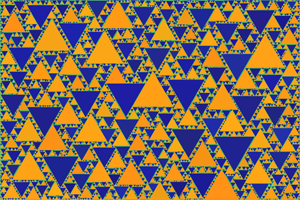
Triangles and nonsquare rectangles have an ordering behavior.
The triangle case has a special feature: If all of the triangles have the same orientation the algorithm fails. If the triangles have alternating "up arrow" and "down arrow" orientations the algorithm runs smoothly.
Nonsquare rectangles are easily "fractalized" by the algorithm if they all have the same aspect ratio, which is not surprising. It turns out that if one allows the aspect ratio (width:height or height:width) to vary from one rectangle to another, keeping the total area the same, the algorithm still smoothly fractalizes them with no changes of c or other parameters. In computer experiments the rectangles all had the same aspect ratio, but even-numbered ones were elongated along X and odd-numbered ones along Y. This gives the algorithm a challenge, since it must find "holes" for elongated shapes. It was found that the algorithm works smootly for aspect ratios from 1:1 to 1:3 (and probably higher).
In the image shown below the aspect ratio was 1:3. The sequence used for the areas began at 10, i.e.
A1=A0/10^c, A2=A0/11^c, ...
with A0 and c adjusted so that the sum to infinity of the areas is just the area A. c=1.26. 60000 rectangles. This family of images has three parameters, rather than the two that one has when the sequence begins at 1. The same equations as above work here, with the Riemann zeta function replaced by the Hurwitz zeta function.
The "X" rectangles are black while the "Y" ones are white. The vacant "gasket" area is red. Study of the image shows that there are "ordered" regions of mostly-white and mostly-black. But even in a mostly-white area there are clusters of black and vice versa. This ordering is produced by the random choice of the algorithm -- constrained by the shape and position of previous shapes.
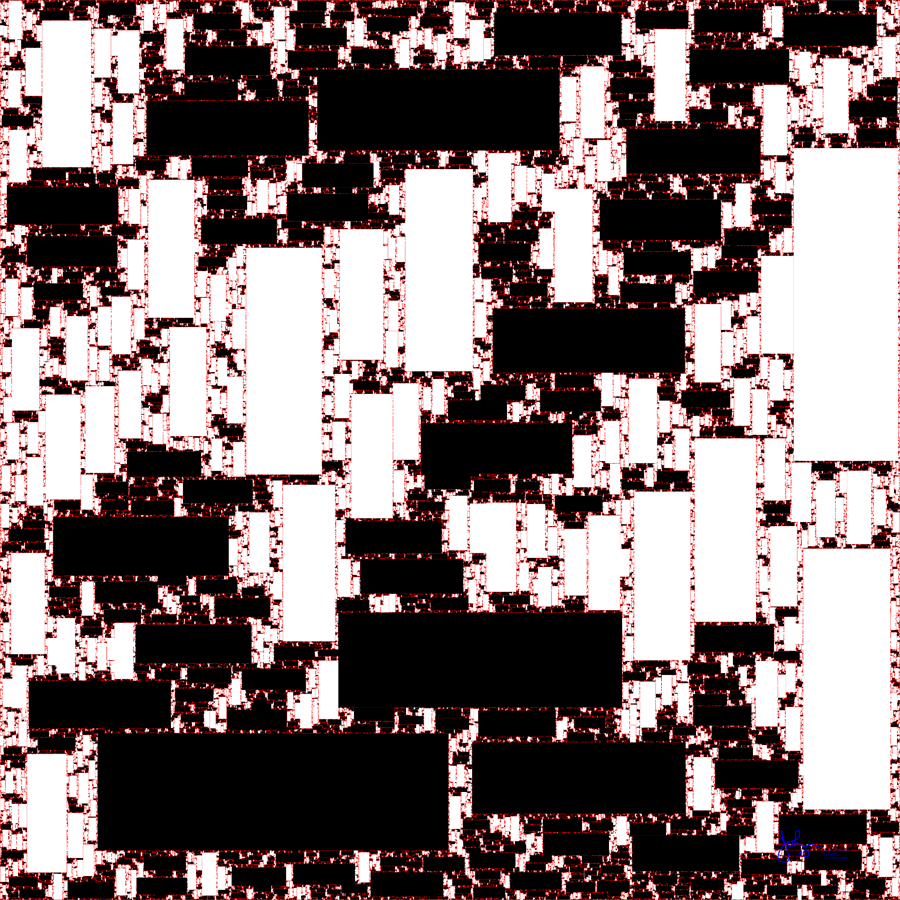
At a small scale one sees the ordering by looking at the small rectangles adjacent to a large one. Most of the small rectangles adjacent to a white one are white, and similarly for the black ones. For a triangle pattern one sees that the "up" triangles are mostly surrounded by "down" ones. For rectangles this ordering property is seen to become more pronounced the more non-square the aspect ratio. This image is blurred, but in the original high-resolution image (60k rectangles) it was clear that the same kind of ordering holds at all length scales. The ordering visibly increases for larger aspect ratios.
Another feature of the algorithm is that vertical rectangles are predominant near the vertical boundaries, while horizontal boundaries have mostly horizontal rectangles nearby.
It is not clear how one should describe this ordering property mathematically.
The curve of cumulative iterations versus i <nit(i)> = n0*i^f was fitted to the rectangle data and gave good straight lines on a log-log plot. The results for several aspect ratios were as follows.
aspect=1.0:1 c=1.26 f=1.289 n0=3.09
aspect=1.5:1 c=1.26 f=1.292 n0=3.10
aspect=2.0:1 c=1.26 f=1.283 n0=3.52
aspect=2.5:1 c=1.26 f=1.287 n0=3.56
aspect=3.0:1 c=1.26 f=1.278 n0=4.13
The value of f is significantly higher than c, which may arise from the use of a sequence not beginning with 1. Within the noise, f is the same for all aspect ratios. The n0 data is somewhat noisier, and shows a mild upward trend. It appears that using more elongated rectangles does not make the algorithm search much longer to find places for new shapes. I found it surprisingly robust.
6. Conjectures -- What Remains to be Done?
It would be interesting if it could be shown that the power laws used here are the only laws which work.
It is noted that available data says that the exponents f and c are the same (within statistical error) for sequences beginning with 1. It would be interesting if it could be shown that the most probable value or the expectation value of f is c in this case.
It would be interesting to clarify the asymptotic behavior of the ratio b defined above as i goes to infinity. This problem does not involve randomness since it depends only on nonrandom calculations of the gasket area, perimeter, and size versus i. This problem intimately involves (various sets of terms in) the infinite series for the zeta function.
The parameter b can be defined for any functional rule Ai = g(i). It can be speculated that near-constancy of b as i goes to infinity is a requirement for any successful algorithm of this kind. In fact, by calculating the b parameter on-the-fly as the algorithm progresses, it might be possible to develop an "adaptive" choice of the next circle size.
The author does not know of any formal scheme for describing the statistical properties and ordering of an object of this kind. Statistical physics has a vast body of theory developed by several generations of physicists since Boltzmann and Gibbs, but that is lacking here. The physics case is greatly aided by the fact that every atom of a given kind is identical to every other. Here the individual elements (shapes) are all different.
It would be interesting to find a rigorous way to characterize and describe the fragmentation of the "gasket".
It would be interesting to determine what classes of shapes can be "fractalized" using this algorithm, and what can't. The algorithm works well for a circle or square (low perimeter-to-area ratio). It also works for nonsquare rectangles of mixed orientation. It fails to work for the equilateral triangle without additional requirements such as differing orientations at each step.
John Shier -- October 2010